Implemented mapping and localization in an indoor environment using information from an IMU and a LiDAR sensor.
Hardware:
The humanoid has a Hokuyo LiDAR sensor product link on its head (the final version of the robot had it in its chest but this is a different version). This LiDAR is a planar LiDAR sensor and returns 1080 readings at each instant, each reading being the distance of some physical object along a ray that shoots off at an angle between (-135, 135) degrees with discretization of 0.25 degrees in an horizontal plane (shown as white rays in the picture). Used the position and orientation of the head of the robot to calculate the orientation of the LiDAR in the body frame. The second kind of observations we will use pertain to the location of the robot. Directly used the (x, y, θ) pose of the robot in the world coordinates (θ denotes yaw). These poses were created presumably on the robot by running a filter on the IMU data (such estimates are called odometry estimates), and due to inherent tracking errors, these poses will not be extremely accurate. More about the hardware in this paper: link.
Coordinate frames:
The body frame is at the top of the head (X axis pointing forwards, Y axis pointing left and Z axis pointing upwards), the top of the head is at a height of 1.263m from the ground. The transformation from the body frame to the LiDAR frame depends upon the angle of the head (pitch) and the angle of the neck (yaw) and the height of the LiDAR above the head (which is 0.15m). The world coordinate frame where we want to build the map has its origin on the ground plane, i.e., the origin of the body frame is at a height of 1.263m with respect to the world frame at location (x, y, θ).
Dataset:
Utilized the data collected from a humanoid named THOR that was built at Penn and UCLA video link. Used 4 different trajectories of the robot in Towne Building at Penn.
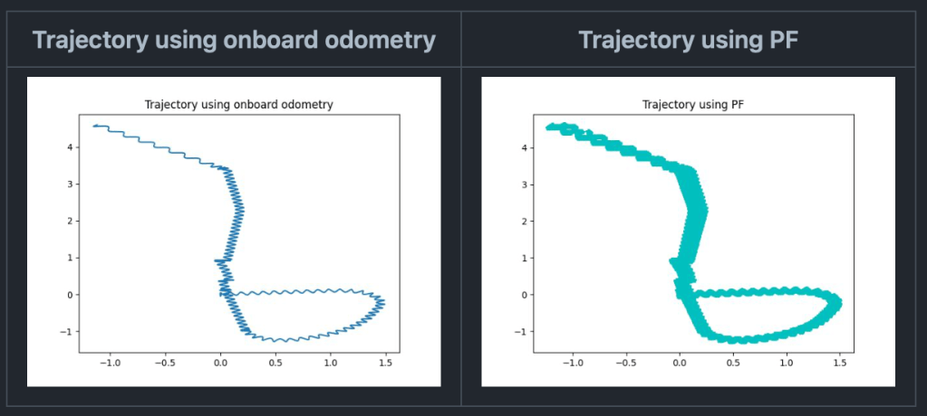
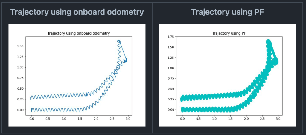
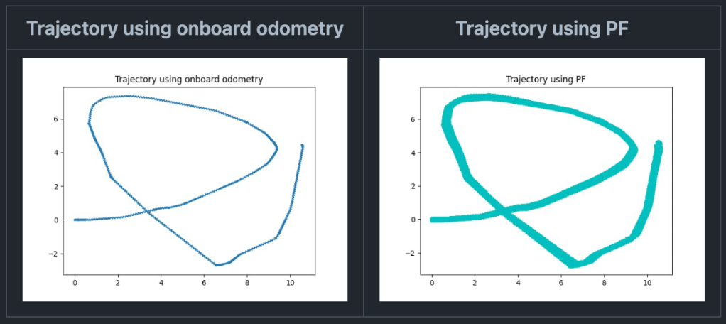
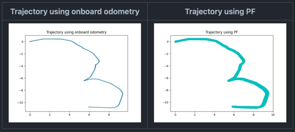
Binarized version of the map with Partical filter plots
Cyan trajectory = Odometry Trajectory
Red trajectory = Trajectory using Partical filter with the largest weight at each time-step
Map 1

Map 2

Map 3

Map 4

Plots for dynamic propagation step:
Map 1
Map 2
Map 3
Map 4