Using Optical Flow the point correspondences and depth are estimated.
More about this is mentioned here.
3D Reconstruction from two 2D images using 2 view SFM:
More about this is mentioned here.
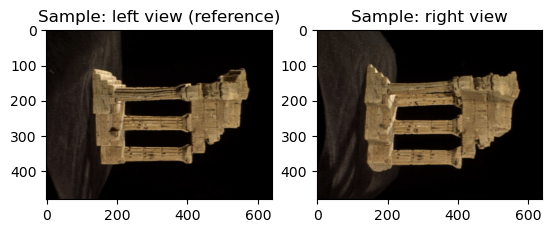
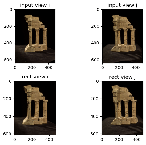
First, computing the right to left transformation and the baseline B. Then, the rectification rotation matrix is computed to transform the coordinates in the left view to the rectified coordinate frame of left view. Since, the images in the dataset are rotated clockwise and the epipoles are placed at y-infinity. Then homography is computed and the image is warped. Zero padding at the border is used and then each left image patch and each right image patch are compared using the SSD kernel, SAD kernel and ZNCC kernel.
L-R consistency: The best matched right patch for each left patch is found.
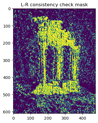
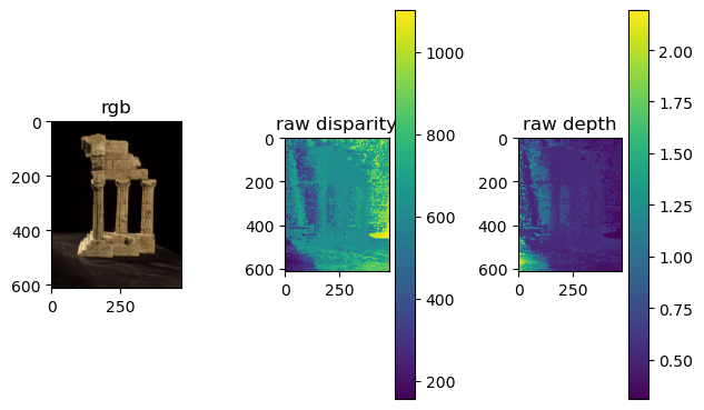
The following disparity map is computed:
Using the disparity map the below Depth map and the back-projected Point Cloud are generated.
Reconstruction using SSD:
Reconstruction using SAD:
Reconstruction using ZNCC kernel:
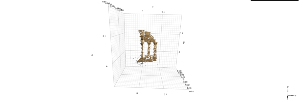
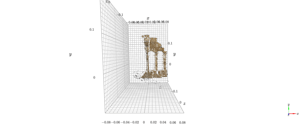
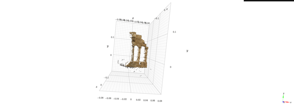
Multi-pair aggregation: full reconstructed point cloud of the temple:
Reconstructing the 3D model from multi view Stereo
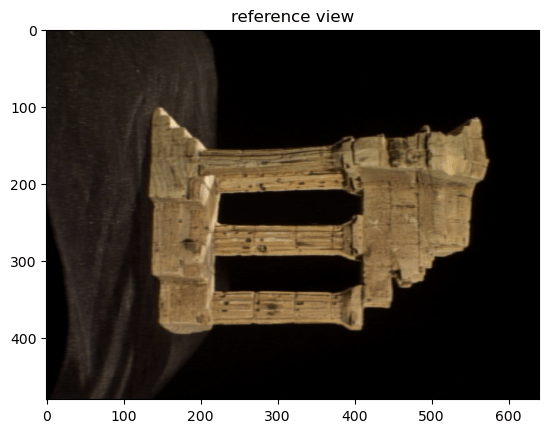
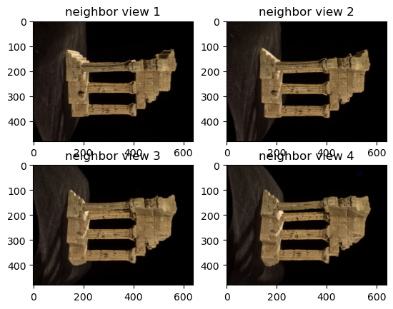
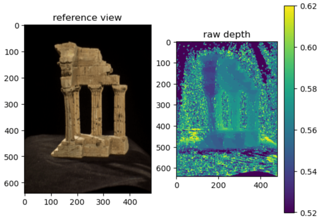
Using 5 different views, choosing the middle-most view as the reference view, the 3D model is reconstructed. The main idea is that a series of imaginary depth planes are swept across a range of candidate depths and the neighboring views are projected onto the imaginary depth plane and back onto the reference view via a computed collineation.
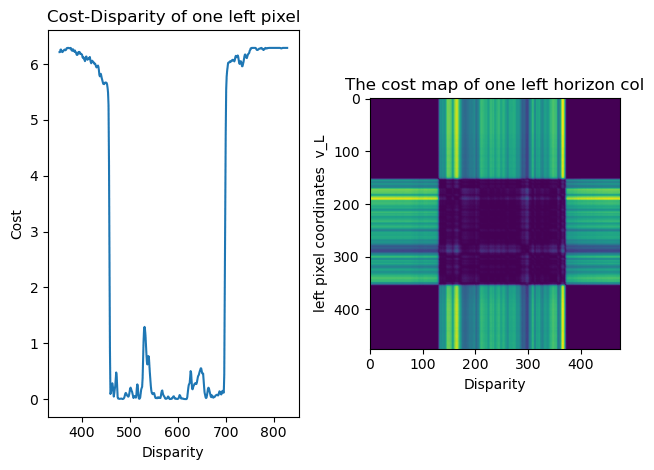
Cost map: The cost/similarity map is computed between the reference view and the warped neighboring view by taking patches centered around each pixel in the images and by computing similarity for every pixel location. At patches with the correct candidate depth, the similarity will be high, and the similarity will be low for incorrect depths.
Cost volume: For each depth plane, the above steps of computing a cost map between the reference view and each of the 4 neighboring views and sum the results of each of the 4 pairs to aggregate into a single cost map per depth plane are repeated. By stacking each resulting cost map along the depth axis, the cost volume is produced.
Depth map: The depth map is extracted from the cost volume ,by choosing a depth candidate and by taking the argmax of the costs across the depths at each pixel.
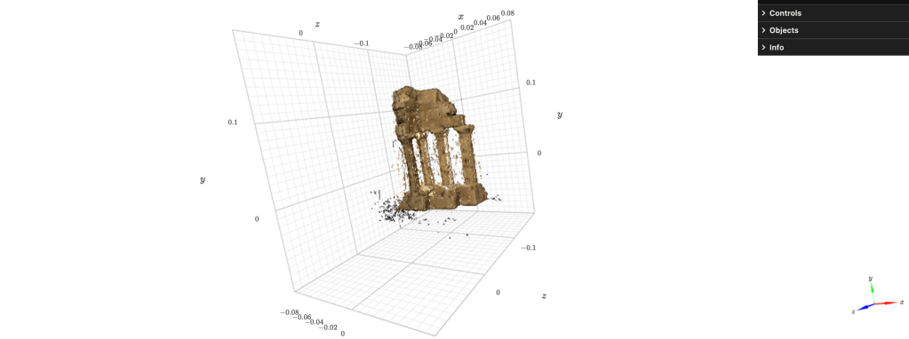
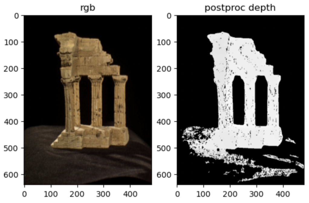
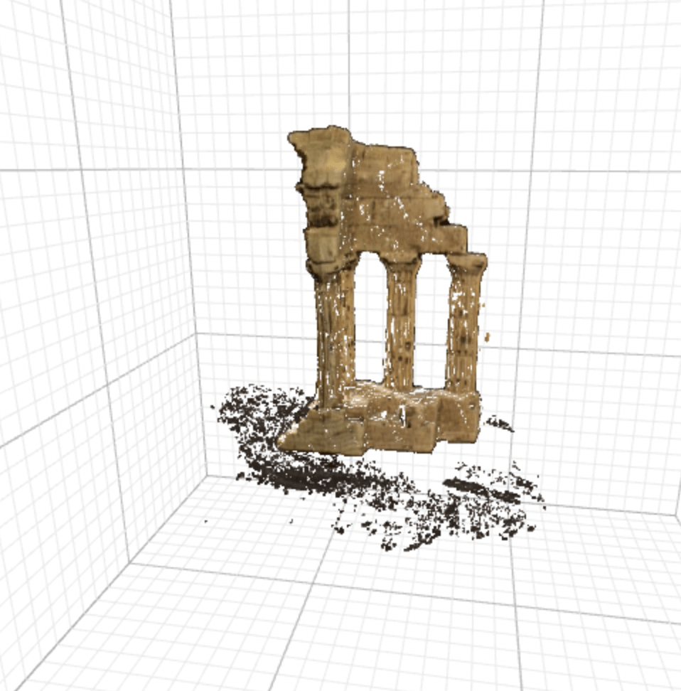
Point cloud: The pointcloud is obtained from the computed depth map, by backprojecting the reference image pixels to their corresponding depths, which produces a series of 3D coordinates with respect to the camera frame.
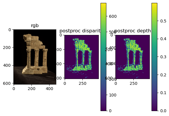
Post-processing: These coordinates are then expressed with respect to the world frame instead of the camera frame. Post-processing is done to get a colorized pointcloud from the depth map by filtering the black background and any potential noisy outlier points.
Code: click here
